
ML & AI: A Predictive Model for Language Family
ML & AI: A Predictive Model for Language Family
Why does my model think Klaus Kinski is Japanese?

In the last post in this series, I criticized some metrics used by data scientists to analyze predictive model accuracy. Judging by my metrics, you didn’t read that post. That’s fine, as it fell prey to some of the vagueness that I hate in both data science and business pedagogy. No one needs a Ted Talk about the importance of setting goals and accomplishing them.
This time, I’ll provide some additional clarity by discussion a specific data science problem. The data for my project sits in my professional portfolio, so I won’t link to it here. I want to keep my Substack life and work life separate, though I do spend quite a bit of the latter’s time on the former.
If this blog existed a decade ago, it would contain dozens of posts about language change, linguistics, and English word etymologies. A couple degrees and and many years of professional work later, my linguistic knowledge has diminished and been replaced more mundane knowledge about data and coding. I still remember a bit though, so I’ll showcase a cool etymology fact before we get to the graphs.
English is a Germanic language, so most English color words match their German equitant. White → weiß (the ß is pronounced like the “ss” in “grass’). Green —> grün ( the ü is pronounced kinda like a mixture between the the “oo” in moon and “ee” in, well, “green”). Blue → blau. Yellow —> gelp (gonna have to trust me on these being similar). Brown → braun. Grey → grau. Black → … schwarz.
Wait, schwarz? What happened here? Turns out, Old English confused a similar word, “swart,” which resembles it’s German sibling. The English “black,” on the other hand, derives from an older term meaning something like “burned.” Another English word shares the same ancestry: bleached! Thus, the word for “black” and the word for “making something the the color opposite to black” share the same origin.
I decided to combine my old and new knowledge bases by creating a model predicts word origins. To do so, I borrowed an etymology dataset from UC Berkeley, and grouped English words (thus far) into four origins: Germanic, Latin, Greek, and Japanese. Germanic words include any word native to English, as well as any borrowed from languages like German or Dutch. Latin refers to words from old-school Latin itself, alongside any from it’s modern children. Greek and Japanese refer to words from, uh, those languages. There’s other word origins in the data, but my models really sucks at spotting Arabic and Indo-Aryan words right now, so I removed them.
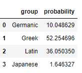
How could a model predict these origins? There’s a couple signs that I would expect a neural network to learn. For example, words ending in “ck” are usually Germanic, while words ending in “ce” usually derive from Latin. We can test if the model discovered these fact by asking it to predict the origin of fake words. Let’s see what my model thinks of “nonsenseck”
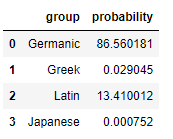
It’s pretty darn sure we have a Germanic word. Just for fun, let’s throw a Germanic “w” in front for “wnonsenseck:”
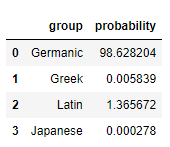
That’s about as Germanic as they get. Lets see what it thinks about “nonsensece:”
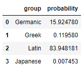
What about the arch-nemesis of the Germanic “w:” the Latin “v?” How does my model feel about “vnonsence?”
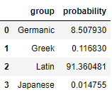
Just for fun, let’s check a more Japanese structured “nonsenska.” I added the fake word looks Latin without it.

Finally, let’s throw a Greek “ph” in front and change one of the vowels to a “y” and create “phnonsyns”
It’s not perfect though, here’s the model’s best shot at “klaus kinski.”
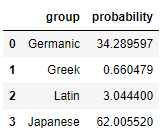
…bruh. Two “k”s? The suffix “ski”? The “au” vowel pair? That looks Japanese to you?
While it’s fun to enter in weird letter combinations and see the model’s output, none of this tells me how well it performs at understanding the English lexicon. To do gauge that, we’ll need to see how it predicts actual English words.
To provide some context, data scientists cut their dataset into a “training” set and a “test” set. In the training set, our model learns the relationship between features (in this case, combinations of letters) and the target (in this case, the word’s origin). We then test this model on our (you guessed it) test set, because we want to ensure that our model can be generalized to data it hasn’t seen before. Following a rule of thumb, I divided 70 percent of my data into training and 30 percent into testing.
From the last 30 percent, I use the mosel to predict the origin for each word. This creates results like the ones above, with a probability of the word falling into each of the four groups. We can also interpret these results as a class prediction by taking the language group with the largest percentage. The class predictions allow us to produce some of the prediction diagnostics discussed in the last post: accuracy, precision, recall, F1 score, and more. I don’t like these metrics, so I won’t discuss them here.
Clarification models produce two types of predictions: probability predictions (e.g. 80% Germanic, 15% Latin, 5% Japanese) and class predictions (e.g. Germanic). I’ll provide a thought experiment to show why we should prefer the former to the latter. Imagine two people create a model that predicts the results of one-on-one basketball games. We then ask those models to predict a game between LeBron James and I. Model one predicts a 99.99% chance of James victory, while model two predicts a 53% chance of the same result. In both cases, the model produces a correct class prediction: a LeBron victory. However, the former model provides a better representation of reality. Diagnostics like the F1 score don’t make this distinction
We also need to consider the purpose for a predictive model. There might be some instances where only the class matters and we don’t care about probability. I haven’t encountered one, but I could imagine a scenario that requires such a model. In my experience, businesses need to know which customers are most likely to churn, which transactions are most likely fraudulent, and other similar questions. A mere class prediction doesn’t help here.
Unfortunately, we run into a bit of a pickle when we try to interpret probability accuracy. Our model produces probabilities, but the real world only produces categories. There aren’t any words that have a 75% chance of being Germanic. A word is either Germanic or it isn’t.
The solve this dilemma, we can use a calibration curve. Calibration answers a question like this one: “For the observations where our model predicts a roughly 10% of being Germanic, are roughly 10% of those actually Germanic?” We can swap 10% for any other number, and you get the idea. In a good model, the predicted probabilities should match their actual proportions in the population. I will arbitrarily bucket my Germanic predictions in groups of 10 percentage points. The first bucket will contain words with a predicted Germanic probability between 0 and 10, the second will contain those between 10 and 20, the third will be 20 to 30, etc. If the model succeeds, 0-10% of the words in bucket one should actually be Germanic, compared to 10-20% in bucket 2, 20-30% in bucket 3, etc. Let’s see the results.
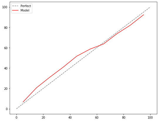
The grey dotted line shows a perfect model. In a perfect model, if the model predicts a 1% of a word being Germanic, 1% of those words should actually be Germanic. If the model predicts a 2% chance of a word being Germanic, 2% of those words should actually be Germanic, and we can continue that logic up to 100%. The closer the predictions sit to the gray line, the better the result. Hence, I think my model performs well since it doesn’t diverge much from the gray line.
While calibration gauges accuracy, we also want to understand the value added from our model. In business, we might prioritize the rankings of the predictions: the most likely to churn, the most likely to be fraudulent transactions, etc. We need lift for that. Lift tells us how much more likely our model is to find positive results (in this case, Germanic words), compared to a base case.
After making predictions, we can sort our data by the probability of word being Germanic. In other words, the first observation will be the word most likely to be Germanic, the second word would be the one second most likely to be Germanic, etc. Now, we can take, say, the top 10% of the data. In a “naive” or “random” model, we would expect the top 10% of the data to contain 10% of the Germanic words. It’s random, so there’s no reason for the percentages to differ. For our model, meanwhile, the top 10% of the data contains roughly 20% of the Germanic words. Thus, for the top 10% of the data, our model proves 2x lift over a random one. We can then plot this ratio for every value from 0-100% to create a lift curve.
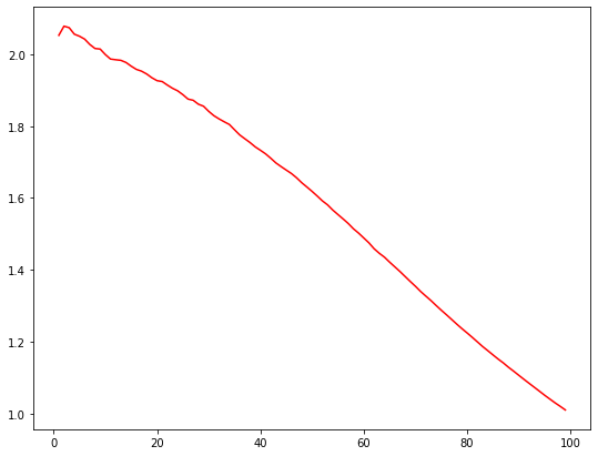
For a naive model, we would obtain a flat horizontal like at 1. It provides no lift over itself. The higher the line stands above 1, the more lift it provides. Lift curves should always decrease, but they usually resemble a, you know, curve. In most data science problems, we analyze “imbalanced data:” data that contains much more of one target than another. Most credit card purchases are legitimate, for instance, so transaction data features a lot more non-fraudulent transactions than fraudulent ones. Our dataset is more balanced (like 50% Germanic words), so we end up with more of a “lift line” than a “lift curve.”
I hope everyone enjoyed some IRL data science! Part 4 of this series will introduce the concept of artificial intelligence, alongside two (quite different) AI models. I can also explain how this predictive model works, if anyone’s interested.
I think it would help the reader if the title is--A model to predict word origins. Is there a list of the word set?
I found four typos. Lemme know if You're interested, M. Klaus.