
Let's Fake Large Effect Sizes
Let's Fake Large Effect Sizes
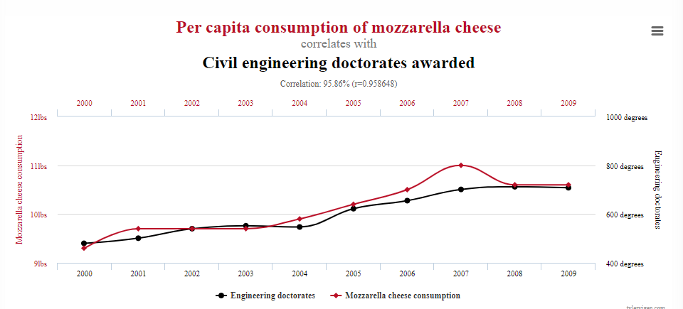
How mozzarella cheese can solve our infrastructure woes

Last time, I p-hacked a randomly generated dataset to find some spurious medical outcomes. This time, I’ll discuss another issue that I’ll discuss effect size rather than statistical significance.
In this article, I will refer to the effect size as the change in one variable associated with a one-unit increase in another variable. For example, a linear regression might find that an additional year of education is associated with an additional $2,000 in annual income. In that case, the effect size for years-of-education would be $2,000.
You might see a study with a small sample size and large effect size. Imagine a study of 40 patients which shows that drinking an additional cup of coffee each day lowers cancer risk by 5%. One might read this and think, “wow, they found that large of an effect in a small sample; that must indicate a really strong result.” However, the opposite is true. In a small sample, you’re more likely to see a large effect size even if the data is totally random. You probably know what’s coming next: we’re going to prove that with data that is, in fact, totally random.
My inspiration came from this page, which shows a series of spurious correlations. Of these, I’m partial towards the relationship between mozzarella cheese consumption and civil engineering doctorates:
Now, let’s find some meaningless effect sizes! Here is the methodology:
I ran 2,000 studies total: 1,000 with a large sample and 1,000 with a small sample
The large sample studies contain 20,000 observations, while the small sample ones only contain 50
Each observation consists of 1) a randomly chosen number of civil engineering doctorates and 2) a randomly chosen value for per capita mozzarella cheese consumption
The “effect size” will refer to the number of civil engineering doctorates conferred by a an additional pound of per capita mozzarella cheese consumption
Of the 2,000 fake studies, here are the effect sizes for both the large and small sample groups:

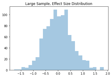
In the large group, we rarely see effect sizes less than -1 or greater than 1. On the contrary, the small sample group regularly shows effect sizes less than -20 or greater than 20!
Of course, most of these results aren’t statistically significant. As such, I will now limit the effect sizes to those with p-values below 0.05. There were 54 such results for the small sample group and 63 for the large sample group. We’d expect more significant results from the latter, since, all else equal, a larger sample size decreases the p-value. For these statistically significant results, I will only show the magnitudes. In other words, an effect size of 8 or -8 would both show up as 8 in the graphs below.

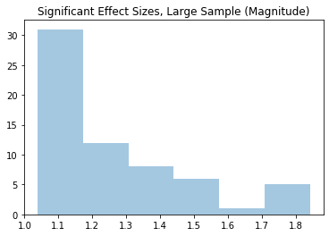
Among the statistically significant results, the large sample only sees effect sizes between 1 and 1.8. Meanwhile, the small sample shows results north of 30.
In short, remember that you should be more skeptical of the effect sizes that come from small-sample studies. Or you can just believe that mozzarella cheese leads to engineering PhDs. It’s up to you.
# Package Imports
import pandas as pd
import numpy as np
import random
import copy
from statsmodels.regression.linear_model import OLS
import statsmodels.api as sm
import seaborn as sns
import matplotlib.pyplot as plt


NUM_OF_STUDIES = 1_000
LARGE_SAMPLE = 20_000
SMALL_SAMPLE = 50

random.seed(0)

large_effect_size = []
small_effect_size = []

large_sig_size = []
small_sig_size = []

for study in range(NUM_OF_STUDIES):
    if study % 100 == 0 and study > 0:
        # Tracking how many "studies" the code has run
        print('study num: ', study)

    # Randomly generating the two large datasets
    cheese = [random.normalvariate(10.5, 2) for _ in range(LARGE_SAMPLE)]
    civil = [random.normalvariate(700, 150) for _ in range(LARGE_SAMPLE)]

    # Taking the first 50 of each to make the small dataset
    cheese_small = [random.normalvariate(10.5, 2) for _ in range(SMALL_SAMPLE)]
    civil_small = [random.normalvariate(700, 150) for _ in range(SMALL_SAMPLE)]

    # Adding a constant
    cheese = sm.add_constant(cheese)
    cheese_small = sm.add_constant(cheese_small)

    # Obtaining the values for the large dataset
    large_model = OLS(endog=civil, exog=cheese).fit()
    large_effect_size.append(large_model.params[1])
    if large_model.pvalues[1] <= 0.05:
        large_sig_size.append(large_model.params[1])

    # Obtaining the results for the small dataset
    small_model = OLS(endog=civil_small, exog=cheese_small).fit()
    small_effect_size.append(small_model.params[1])
    if small_model.pvalues[1] <= 0.05:
        small_sig_size.append(small_model.params[1])

# Get Number of Significant Results
print('Significant results, small sample: ', len(small_sig_size), ';',
      'Significant results, large sample: ', len(large_sig_size))

#Plot Effect Size Distributions

plt.title('Small Sample, Effect Size Distribution')
print(sns.distplot(small_effect_size, kde=False))

plt.title('Large Sample, Effect Size Distribution')
print(sns.distplot(large_effect_size, kde=False))

#Plot Effect Size Distributions among Statistically Signiifcant Results

plt.title('Significant Effect Sizes, Large Sample (Magnitude)')
print(sns.distplot([abs(_) for _ in large_sig_size], kde=False))

plt.title('Significant Effect Sizes, Small Sample (Magnitude)')
print(sns.distplot([abs(_) for _ in small_sig_size], kde=False))
There was one spurious correlation I liked on his website a while back, something about being killed by a mattress. I couldn’t find it just now though.
There’s so much nonsense with effect sizes out there. Pretty much any health or nutrition research described in the mainstream news, if you figure out who wrote the original research and look it up, is so meaningless as to be trivial.
Back when red wine was supposed to be good for you, I think you’d have to drink 3000 glasses a day (or something) to see an effect. Or it’s similar to saccharine causing cancer in mice, who drank the equivalent of hundreds of diet sodas per day for life.
But people read red wine is good for you and start drinking it even if they like beer better, or they switch artificial sweeteners to something that’s probably even worse.
Health science reporting is atrocious!!